Photo by Javier Allegue Barros on Unsplash
Calibrating Machine Learning Models: What, Why and How?
Safa Abbas | 11th november 2022
Humans when making a statement or decision have a gauge of certainty, we use language to express how confident we are about what we are talking about. In business, to trust and use modeled data, data processing and modelling should be transparent and explainable. If businesses are to make important decisions about investment, or risk, they have to be able to understand how models work and how models come to the final scores they see.
In machine learning we can use different methods to quantify the confidence of our predictions. The most common way of representing a confidence score is a decimal number between 0 and 1 (often represented as percentages), other methods include a set of expressions (low, medium and high) or a number between 0 and infinity.
Confidence Scores and Probability
When discussing performance of models with clients and stakeholders, confidence scores are a way of communicating the likelihood of an input falling into different classes (probability of an event according to the trained model). For example, a model predicting whether a piece of text is relevant or not relevant to a client outputs a prediction of not relevant with a probability of 70%. This doesn’t mean that 70% of the text is not relevant, more that the model thinks that it is 70% likely to be not relevant and 30% will be relevant based on the training of the model. However, different models produce confidence scores in different ways and this can make them confusing to end-users and clients. Some will output a probability, others i.e logistic regression will output an “odds ratio” which is used to determine the strength of association between two events.
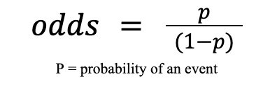
These technical differences can be difficult to explain to clients, and cause confusion when comparing outputs from different models, especially if the models produce confidence scores using different scales such that a score of 0.7 could mean wildly different things coming from two different models. For example:
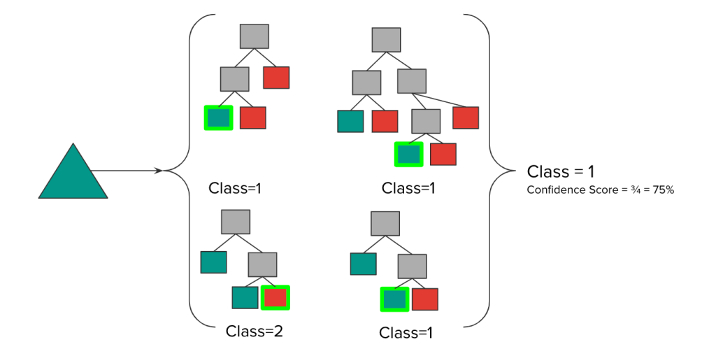
- For a random forest the standard probability estimation method is called “voting”. The proportion of trees that predict a class k when observation x is passed down the tree. Other methods include regression, where the predictions are an average over the trees for a given prediction.
- Neural networks for multi-class problems commonly use softmax activation to calculate the relative probabilities
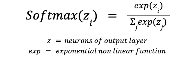
- The values from non linear exponential function are divided by sum of exponential values, this normalises the values which are then converted to probabilities. These values are asymptotic the larger the values from the network, meaning confidence can jump from really low to really high .
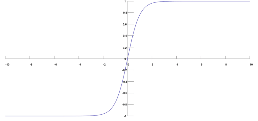
Graph showing soft max distribution.
The histograms below are from the scikit learn documentation for calibration. They show the number of samples in each probability bin, displaying behaviour of different classifier models.
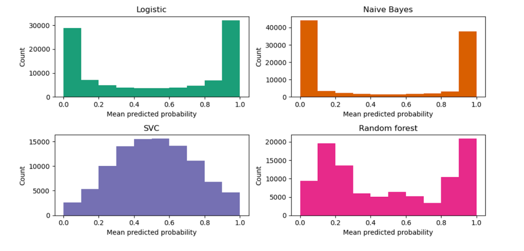
Probability distribution for different classifiers
So different models produce a probability which is calculated in different ways, and represent different things. Therefore, confidence scores from different models cannot be directly compared. This can be challenging for end-users to understand. For example, they may want to know why identical class predictions made by a random forest model and a neural model have wildly different confidence scores and may be inclined to “trust” the more confident model.
As the probabilities or probability-like scores predicted by the models are not calibrated, they may be overconfident in some cases and under-confident in other cases. This depends on the class distribution in the training dataset. Significant imbalance in the training set may result in biassed predicted probability distributions that over-favor predicting the majority class. By calibrating models, we can ensure that the output of these models better reflects the likelihood of true events.
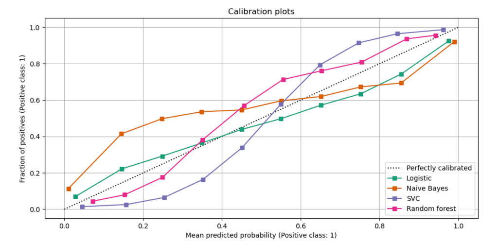
Graph from scikit learn documentation
Worked Example
Imagine we have a bowl of fruit and we are trying to classify each fruit to a name. The bowl has 15 apples, and 5 bananas. If we train a model to predict each of them the bananas would have a really low confidence/probability score, because the classes are unbalanced. When modelling with unbalanced data, the model will have a bias towards the majority class.
For example if we are to pick a fruit from the bowl randomly, we have a higher chance of picking an apple, because there are more of them in the bowl: 75% of the bowl is made up of apples and the other 25% is bananas.
In a calibrated model we would expect the frequency distribution of the model outputs for a randomly sampled set to approximately match that of the “real world” distribution.
Experiment
We often use random forest as our baseline model, and we apply probability calibration. We have shared the code for this experiment here so that readers can have a go at running it themselves.
In this experiment, we use Platt Scaling Calibration, a simple method that was originally developed to scale the output from a SVM to probability values but which can be applied more broadly to a variety of models. It involves learning a logistic regression model to perform the transform of scores to calibrated probabilities. Platt scaling also has the advantage of not needing large amounts of training data (compared to the relatively more complex isotonic regression calibration method which can yield better results if enough data is available).
We ran an experiment to understand the effects of calibration on a multi-class random forest classifier on a publicly available kaggle dataset that maps companies to the sector that they operate in. We use the text description from the meta_descriptions column in the dataset to predict the value in the Category column.
The original dataset consists of 73k companies across 13 sectors/classes which we randomly down-sample to 7.3k records to create our simple baseline model for this experiment.
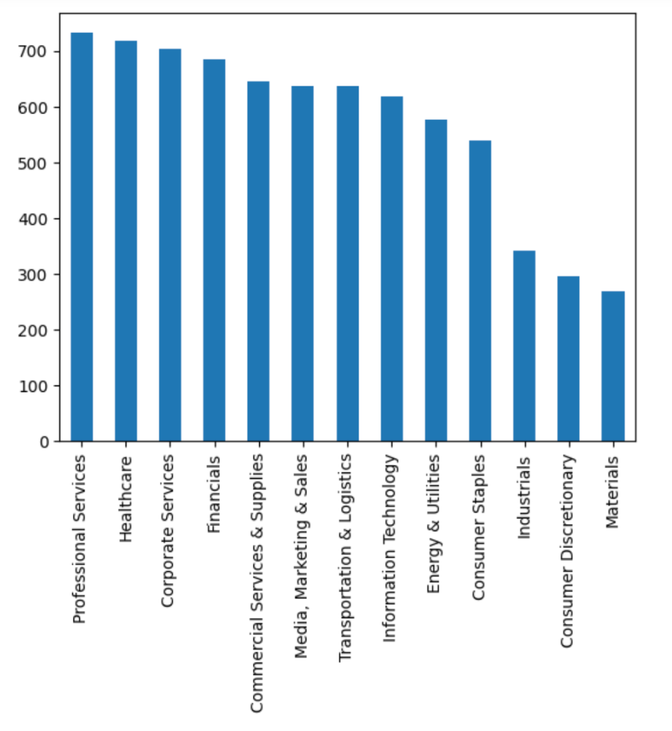
Graph showing amount of company data per sector
After removing the missing company descriptions we trained random forest models with and without calibration to compare the effects of calibration.
Calibration must be done on a data sample that was not used for training to avoid biassing the model. In our experiment, we use the CalibratedClassifierCV implementation from scikit-learn which automatically trains an ensemble of calibrated models which are used to produce an ensemble of calibrated models on different subsets of the training data (in a workflow similar to cross-fold-validation). When used to predict a label for new, unseen data the output from the model is an average of the probabilities taken across the ensemble.
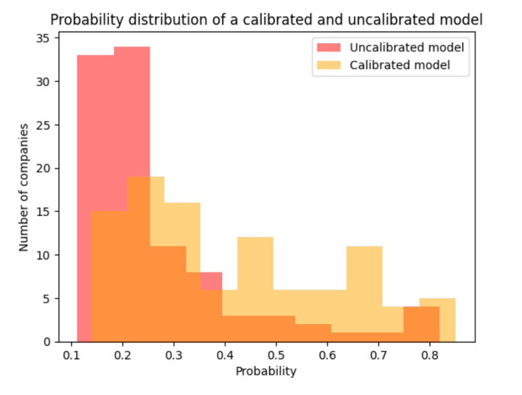
The graph above shows the probabilities of the top predicted sector for a sample of 100 companies that we tested our model on, from each model. The uncalibrated outputs tend to have relatively low confidence scores (reflected by the large cluster of results in the 0.1–0.3 region of the graph) — this is a reflection of the way that Random Forest ensemble models work as discussed above. The calibrated model has a more evenly spread probability distribution which gives a better reflection of the real spread of probable labels in the dataset.
Conclusion
Different ML model types can produce drastically different confidence distributions across their labels even when trained on the same task and this can often be very confusing for non-technical users. For example, users may be concerned about why their Random Forest model is never that confident even when it’s right or why a neural model is so confident even though it got an answer completely wrong.
It is important for end users to understand that model confidence is distinct from model accuracy (and that, like humans, models can be confident and still be wrong). However, Calibrating ML Models is a way to make the confidence scores that they produce better reflect the probabilities of real life events and make the results produced more understandable and relatable to lay-users. They can also provide a way to make confidence scores from different models trained to complete the same task more consistent and less jarring for end users who may be comparing their behaviour.


